Small-Dictionary LCA Sparse Coding for Low-Power Pattern Recognition in Edge Devices
Sparse coding is one such algorithm that has been successful for a variety of applications such as face recognition [@wright2009sparse] and visual tracking [@zhang2013sparse] and has now also found use in energy harvesting context sensing [@xu2018keh]. While there are a variety of algorithms that exist to obtain sparse representations, an algorithm based on competing neurons, the “locally competitive algorithm” (LCA) is particularly promising for use in edge computing due to its compatibility with the memristor crossbar architecture, on which it has been implemented before [@sheridan2017sparse]. In contrast with popular neural networks that do MAC operations with many weight matrices for each neuron on the previous layer, sparse coding in LCA has the potential to be effective with a single crossbar for the dictionary, reducing concerns about memristor variation and scaling problems.
Here, accuracy-energy/size tradeoffs with LCA sparse coding parameter selection, choices of dictionary sizing, and number of quantization levels were explored in anticipation of challenges in the crossbar implementation stemming from quantization, memristor variation and energy constraints.
In the increasingly more popular paradigm of edge computing, information processing takes place not only in powerful servers in center nodes but also in the edges of a network. This allows networks of IoT devices like wireless sensors designed for low-power operation tasks to save even more energy by avoiding energy expensive transmission over multiple hops or long distances.
To evaluate the tradeoffs, sparse coding is used to classify 5 different gestures inferred from the energy harvesting response of a solar cell, synthesized using SolarGest [@ma2019solargest] with the parameters outlined in Table 1{reference-type=”ref” reference=”solargest parameters”}. Here, the current waveforms generated were subsampled into feature vectors of length \(128\). In the end, we produced an LCA sparse coding scheme able to classify 5 different gestures from the current waveform of the solar cell above which these gestures are made to 100% accuracy with only 2 LCA iterations in a \(128\times50\) dictionary matrix.
Classification using LCA
Sparse coding attempts to represent an arbitrary vector \(x\) by representing it as a linear combination of a set of basis functions \(D\), called the dictionary. The choice of basis functions can vary. They can be obtained from standard bases, can be completely random, or made/learned from training feature vectors. The objective of sparse coding is to represent \(x\) in terms a vector of coefficients \(a\) (called the sparse representation) such that \(x=Da^{T}\), but with the constraint that \(a\) be sparse. This can be formulated as the following:
\[min_{a}(|x-Da^{T}|_{2}+\lambda|a|_{0})\label{eq:1}\]where \(|\cdot|_{2}\) and \(|\cdot|_{0}\) are the \(L^{2}\) and \(L^{0}\) norms, terms which prioritize reconstruction accuracy and sparseness respectively. This optimization problem is non-convex and NP-hard. The LCA is a biologically inspired algorithm for approximating the solution \(a\) [@rozell2008sparse]. In the LCA, dictionary elements are modelled as leaky neurons with membrane potentials. The membrane potential \(u\) of an LCA neuron can be described by the difference equation [@sheridan2017sparse]: \(u_{n+1}=\frac{1}{\tau}(-u_{n}+(x-Du_{n}^{T})^{T}D+a_{n})\label{eq:2}\) \(a_{n}=\begin{cases} u_{n} & ifu>\lambda\\ 0 & otherwise \end{cases}\)
Governed by the parameters \(\tau\) and \(\lambda\), the change in the potential \(u\) is proportional by \(1/\tau\) to three terms: its size \((-u)\), its similarity to the input \((x^{T}D)\) and inhibition from similar neurons \((a(D^{T}D-I_{n}))\) where \(D^{T}D-I_{n}\) is the neuron similarity matrix. If a neuron’s potential \(u\) is above the threshold \(\lambda,\) it is deemed active, and it starts contributing to the inhibition term. We use the hard thresholding function for the thresholding Here for simplicity. The compatibility of the LCA with memristor crossbars stems from the fact that in this algorithm, the only matrix that is being used is D and only with matrix-vector multiplications.
Compression using sparse coding is simple, since the values and indexes of the nonzero sparse coefficients can simply be taken as the compressed signal. Classification can be done using sparse coding by appending multiple dictionaries learned for different classes together. After learning each class dictionary \(D_{i}\) for class \(i\), the global dictionary is then made by concatenating the class dictionaries \(D=[D_{1},D_{2},...,D_{N}]\) for \(N\) classes. The usual method to infer the class of \(x\) from \(a\) is called minimal subspace search (MSS). In MSS, given the sparse representation \(a\) from the global dictionary, the signal is reconstructed using only coefficients associated with each class dictionary- and the predicted class is that of the class dictionary that produces the minimum reconstruction error (residue). Getting the residue for MSS is too computationally expensive to do on edge devices, even with the help of memristor crossbars, and hence we opt to just take the class of the largest sparse coefficient \(argmax(a)\). Good classification accuracies are obtained despite this, and so it is shown that this scheme can be enough for the gesture classification done Here- indicating possible viablity for other EH sensing applications as well.
- ::: {#solargest parameters}
- Parameter Mean StDev
- ————————————— ————– ———-
- Hand Diameter \(9.72cm\) \(1.14cm\)
- Hand Pos Low \(2cm\) \(0.1cm\)
- Hand Pos High \(10cm\) \(1cm\)
- Gesture Speed \(20cm/s\) \(1cm/s\)
- Hand Height (for horizontal gestures) \(5cm\) \(1cm\)
- Solar Cell Radius \(2cm\)
- Light Intensity \(200lux\)
- Solar Cell Current Density \(7mA/cm^{2}\)
-
SolarGest Input Parameters with Hand Size Statistics taken from Chia et al. [@chia2020anthropometric] :::
A total of 3000 current waveforms were generated using SolarGest containing 5 gestures, 500 of which were used as the training set and the rest were used as the test set. The class dictionaries \(D_{i}\) were learned using basis pursuit denoising (BPDN) in the SPORCO software [@wohlberg2017sporco]. The global dictionaries hence had a total of \(K*Nclasses\) bases, where \(N\) is the number of classes and \(K\) is the number of bases in a class dictionary. A total of 4 global dictionaries with \(K=150,50,25,10\) were used, along with an unlearned dictionary containing the test vectors and a completely random dictionary.
Results
 {#sample sparse code width=”\linewidth”}
Compressive Sensing
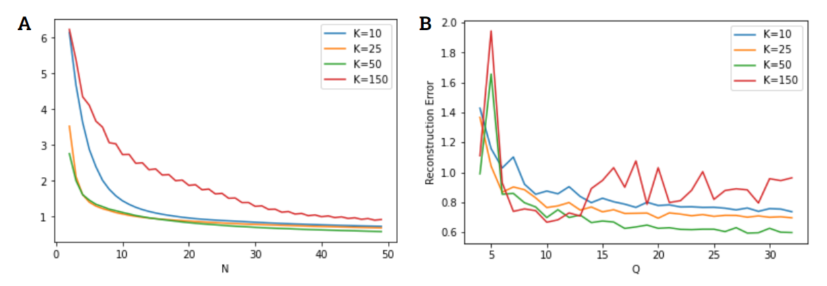
In compressive sensing, the results show that a dictionary as overcomplete as possible is better for the same number of operations and generally for any number of quantization levels.
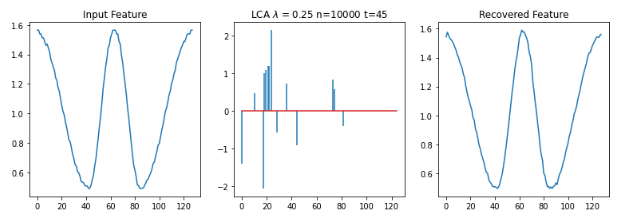
Shown in Figure 2{reference-type=”ref” reference=”reconerror”} is a sample feature reconstruction of various gestures. The LCA fails to converge (it can diverge in discrete time, despite stability in continuous time) to a solution using either the untrained dictionary containing only the training feature vectors or the random dictionary for the parameters shown. For the trained dictionaries, the LCA can settle into a good sparse representation for all \(K=10,25,50,150\) where \(K\) is the number of dictionary elements per class (albeit with a bit of difficulty with the \(K=150\) dictionary).
Dictionaries with less elements generally lead to more reconstruction error for the same number of iterations, as shown in Figure 2{reference-type=”ref” reference=”reconerror”} (a). However, introducing too many elements will introduce a lot of unnecessary neurons to the code whose feature space (the loose set of feature vectors that will activate it strongly) will overlap with each other, introducing oscillatory behavior in the LCA and generally poorer reconstruction. While overcomplete dictionaries should theoretically allow better sparse reconstructions, the dynamics of the LCA system in discrete time introduces mistakes in single iterations that are more significant the more competition there is (more similar receptive fields between the LCA neurons).
| {#reconerror width=”\linewidth”} |
When the dictionaries are quantized, the lower the quantization number the lower the reconstruction accuracy gets for a specific number of iterations. This reconstruction accuracy does not get better over more iterations, resulting in a sort of steady-state error, as seen in Figure 2{reference-type=”ref” reference=”reconerror”} (b). The quantization can sometimes randomly be better for the reconstruction, and \(K=150\) having more elements is subject to this effect the most while the others can be observed to get less random fluctionations as the dictionaries get smaller.
Pattern Recognition
Using as few iterations for the LCA as possible is ideal to lower the energy consumption of the computation in a memristor crossbar. From equation [eq:2]{reference-type=”ref” reference=”eq:2”}, each iteration of the LCA only needs two vectors to be multiplied to the dictionary \(D,\) and hence, the number of crossbar operations is twice the number of iterations \(c=2n\). Furthermore, a dictionary as small as possible is also ideal for a smaller crossbar, which also directly reduces the energy consumption of the computation.
Lower \(K\) and \(Q\) result in better classification accuracies suggesting that concatenating dictionaries as undercomplete (as low \(K)\) as possible for each class is ideal for classification using LCA. It may be that by reducing the number of dictionary elements, the learned elements are forced to be more orthogonal to each other, increasing the discriminative ability at the cost of reconstruction accuracy (for which overcomplete dictionaries are better, since infinite sparse solutions exist) as was found in the previous section.
Optimal combinations for \(\tau\) and \(\lambda\) can be seen in the grid sweeps in Figure 3{reference-type=”ref” reference=”fig:-colormaps-of”}. While for some dictionaries the classification accuracies are already too high (lots of \(\tau-\lambda\) lead to 100% accuracy), optimal combinations of \(\tau-\lambda\) as a function of \(n\) and \(Q\) exist for the other dictionaries. The derivation of analytical expressions for guidelines of optimal combinations from this empirical data is possible, the derivation of which may be good for more difficult classification tasks.
These maps are non-concave, since many local maxima can be found through the grid search. Thus, the use of gradient ascent and the like will be subject to many local maxima, and not be guaranteed to reach the optimal parameters. Despite that, stochastic gradient ascent still tends to reach a set of parameters that give near-optimal accuracy for any \(n,K,Q\) combinations, given good guesses for the starting points which tend to be \(\tau\in(20,30),\lambda\in(0.1,0.3)\).
- ::: {#maximums}
- Dictionary N \(\lambda,\tau\) Accuracy
- ———— — —————————– ———-
- \(K=150\) 2 \((0.234,25.873)\) \(0.67\)
- 5 \((0.217,12.381)\) \(0.666\)
- \(K=50\) 2 \((0.222,23.492)\) \(0.73\)
- 5 \((0.094,25.079)\) \(0.772\)
- \(K=25\) 2 \((0.117,29.841)\) among many \(1\)
- 5 \((0.050,21.111)\) among many 1
- \(K=10\) 2 \((0.122,51.270)\) among many 1
- 5 \((0.261,59.206)\) among many 1
-
Maximum Accuracies found for grid search in Figure 3{reference-type=”ref” reference=”fig:-colormaps-of”} :::
 {#fig:-colormaps-of width=”\linewidth”}
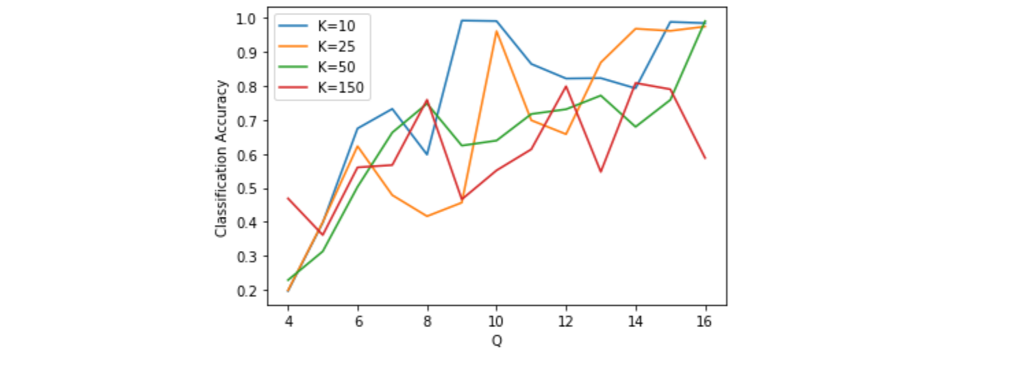
In general, lower \(K\) dictionaries perform better against less quantization levels. However, it can be seen from Figure 4{reference-type=”ref” reference=”acc for diff q n=00003D2”} that, holding\(K\) constant, less quantization levels can be better for the classification accuracy. In particular, it can be noted that \(K=10\) and \(25\) plummet after \(Q=10\) and \(9\) respectively. After \(Q=8,\) all the dictionaries work suboptimally. This may be a somewhat random contribution where some quantizations are coincidentally better.
 {#acc for diff q n=00003D2 width=”\linewidth”}
The high \(K\) dictionaries also benefit from more iterations as seen in Figure 5{reference-type=”ref” reference=”acc vs n”}, while the lower \(K\) dictionaries actually suffer with higher \(n\), worse in the middle ranges. This can likely be due to the fact that a high \(K\) allows for more coincidentally activated elements of the wrong class, while more quantized (lower \(Q\)) dictionaries are more susceptible to a sort of steady state error as the number of iterations increase.
\(K=150\) performing better for odd iterations may be due to oscillation in the LCA output, where the input \(x\) tends to activate a specific set of neurons \(a_{x}\subset a\), but these neurons are extremely similar to each other and thus tend to beat each other down through inhibition in the very next cycle. This is removed by decreasing \(K,\) since forcing the BPDN dictionary learning algorithm to work with less elements forces it to make the elements more dissimilar.
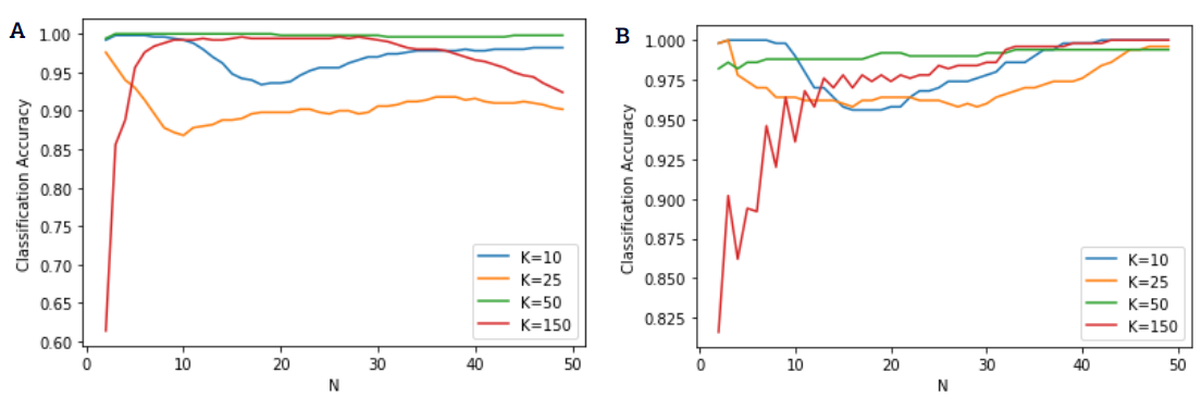 {#acc vs n width=”\linewidth”}
Effects of Conductance Variation on Pattern Recognition
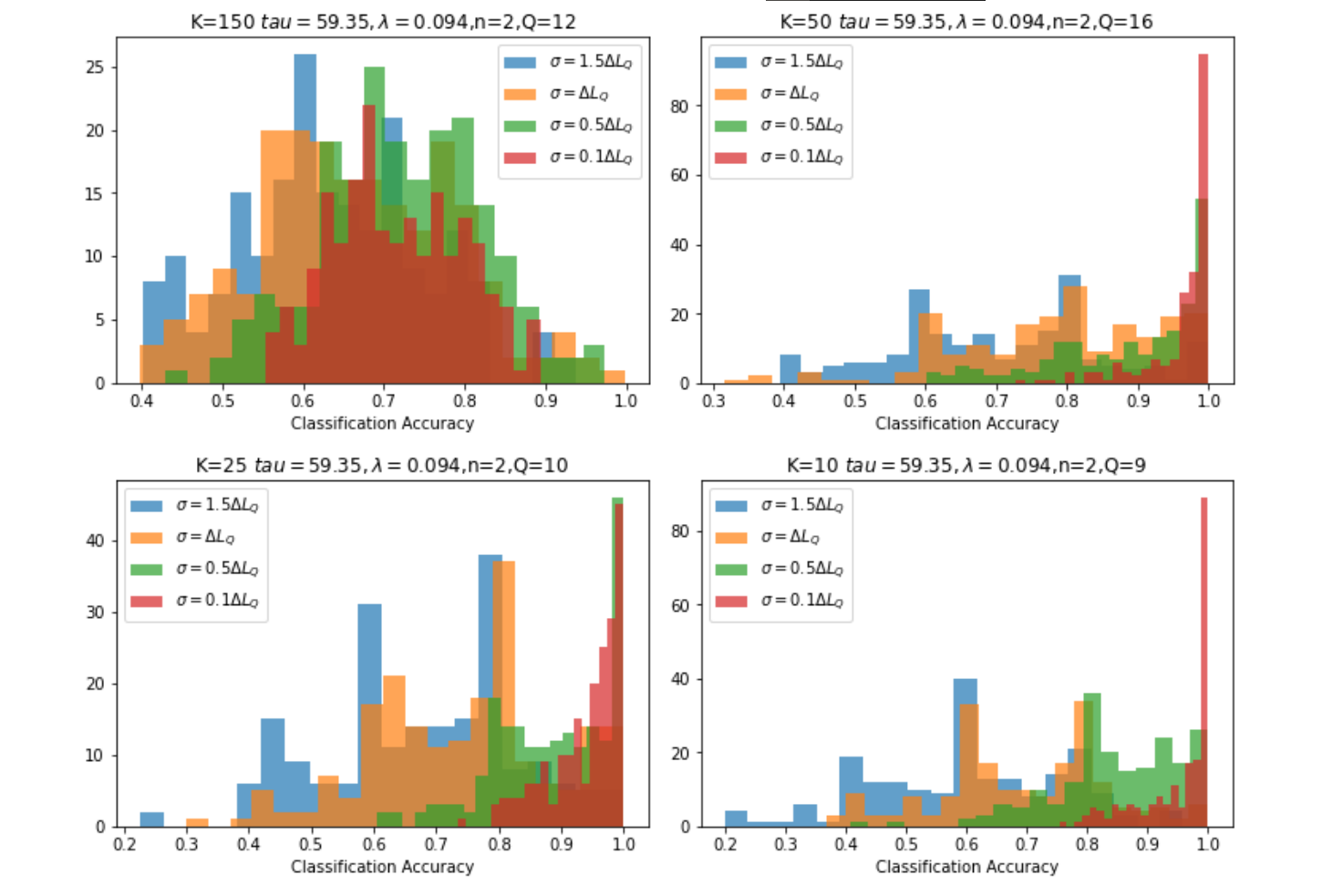
The standard deviation \(\sigma\) of the conductance of a memristor crossbar is around the difference of two conductance levels in Sheridan et al. [@sheridan2017sparse], and so that is used as the reference for the conductance variation, henceforth noted as \(\Delta L_{Q}\). Shown in Figure 6{reference-type=”ref” reference=”hist”} are the histograms of each dictionary on the lowest quantization level \(Q\) where they achieve great accuracy results, since a low \(Q\) is ideal for memristor fabrication and write methods.
Standard deviations as much as \(\Delta L_{Q}\) can render the scheme unusable, and it is visible that even a \(0.1\Delta L_{Q}\) variation can affect the accuracy to as low as \(80\%\), which needs to be noted when choosing the memristor to implement the scheme with. Fortunately, the scheme is shown to work to very low \(Q\), which may let fabricators optimize the memristors for less variation.
Visually, \(K=10\) gives the best distribution, with the highest number of still-100% accuracies at \(0.1\Delta L_{Q}\), while having waveforms similar to \(K=50\) and \(25\) in the other standard deviations. While \(K=150\) is showing terrible results here, that is because it is being run at \(Q=12,\) since its best accuracies can only be obtained at \(n\) higher than 2 (as seen in Figure 5{reference-type=”ref” reference=”acc vs n”}).
 {#hist width=”\linewidth”}
Conclusion
We showed that sparse coding with LCA can be used as a machine learning algorithm suitable for use in edge devices such as energy harvesting wireless sensor nodes if paired with memristor crossbars. A 100% classification accuracy was achieved on the solar cell gesture dataset with only 2 iterations of the LCA on the \(K=10\) dictionary: only \(4\) usages of a small \(128\times50\) crossbar, showing great promise of extremely low energy/classification while avoiding the problems present in large scale crossbars. Subsampling the waveforms smaller than \(128\) can potentially knock the size of this crossbar down to a smaller scale, avoiding scaling problems with big crossbars.
Larger dictionaries with more elements tend to be better for compression, because they allow for better signal reconstruction. However, smaller dictionaries are much better for classification. Smaller dictionaries are also more robust against quantization, showing great classification accuracies to as low as \(Q=9.\) The accuracies can, however, vary significantly with conductance variations on the memristors. This trades off with the precision to which conductances need to be written onto the memristors, increasing the energy required.
Using a quantization-aware dictionary learning algorithm like QK-SVD may further increase classification accuracies for less quantization levels. Small-dictionary LCA sparse coding still also needs to be proven effective for more difficult EH classification tasks, such as with noisy data from piezoelectric harvesters. Future work exploring the effectivity of small-dictionary LCA scheme for other EH context sensing tasks or for its already-proven face recognition and visual tracking capabilities is recommended.